A Tour of the flatsurf Suite
The flatsurf software suite is a collection of mathematical software libraries to study translation surfaces and related objects.
The SageMath library sage-flatsurf provides the most convenient interface to the flatsurf suite. Here, we showcase some of its major features.
Defining Surfaces
Many surfaces that have been studied in the literature are readily available in sage-flatsurf.
You can find predefined translation surfaces in the collection translation_surfaces.
from flatsurf import translation_surfaces

S = translation_surfaces.cathedral(1, 2)
S.plot()
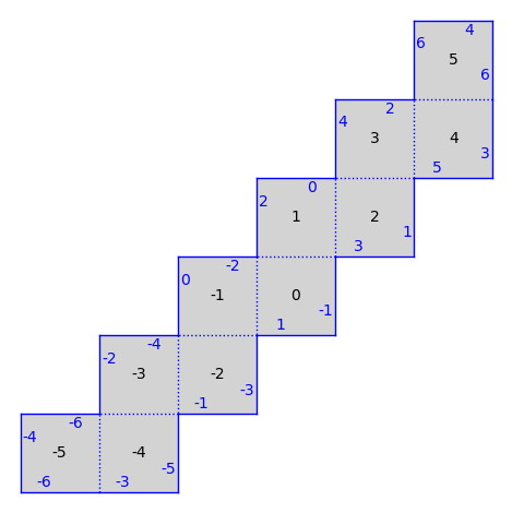
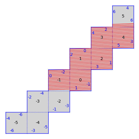
There are also infinite type surfaces (built from an infinite number of polygons) in that collection.
from flatsurf import translation_surfaces

S = translation_surfaces.infinite_staircase()
S.plot()
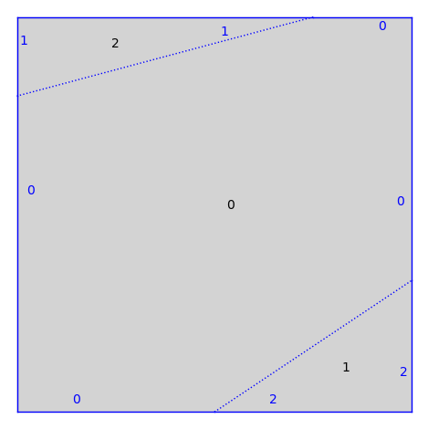
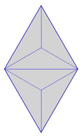
Some more general surfaces where the gluings are dilations are defined in the collection dilation_surfaces.
from flatsurf import dilation_surfaces

S = dilation_surfaces.genus_two_square(1/2, 1/3, 1/4, 1/5)
S.plot()
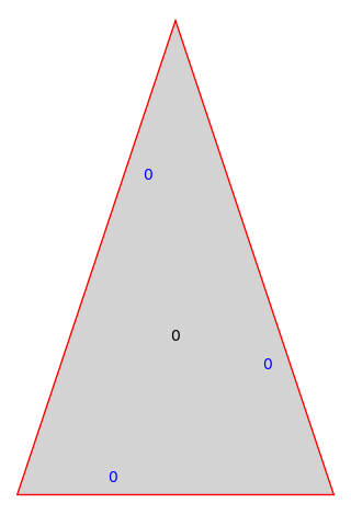
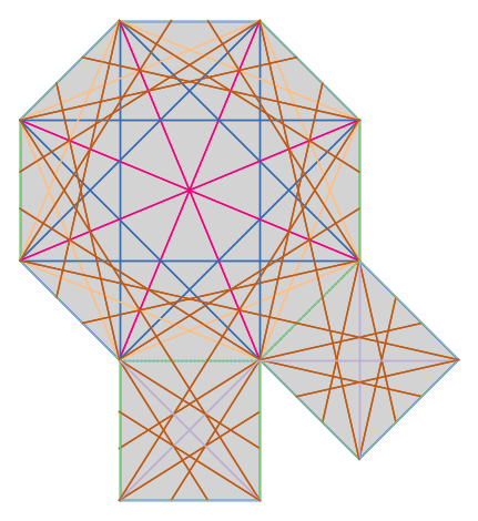
Even more generality can be found in the collection similarity_surfaces.
from flatsurf import Polygon, similarity_surfaces

P = Polygon(edges=[(2, 0), (-1, 3), (-1, -3)])
S = similarity_surfaces.self_glued_polygon(P)
S.plot()
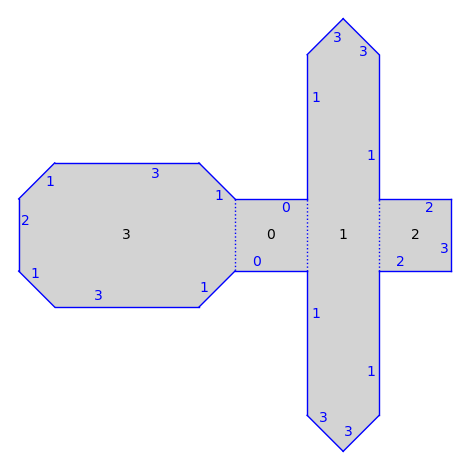
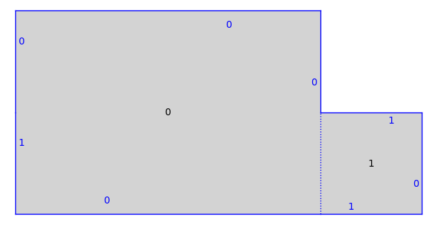
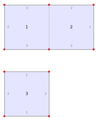
Building Surfaces from Polygons
Surfaces can also be built from scratch by specifying a (finite) set of polygons and gluings between the sides of the polygons.
Once you call set_immutable(), the type of the surface is determined, here a translation surface:
from flatsurf import MutableOrientedSimilaritySurface, Polygon

hexagon = Polygon(vertices=((0, 0), (3, 0), (3, 1), (3, 2), (0, 2), (0, 1)))

square = Polygon(vertices=((0, 0), (1, 0), (1, 1), (0, 1)))

S = MutableOrientedSimilaritySurface(QQ)
S.add_polygon(hexagon)
S.add_polygon(square)

S.glue((0, 0), (0, 3))
S.glue((0, 1), (1, 3))
S.glue((0, 2), (0, 4))
S.glue((0, 5), (1, 1))
S.glue((1, 0), (1, 2))
S.set_immutable()

print(S)
S.plot()
Translation Surface in H_2(2) built from a square and a rectangle
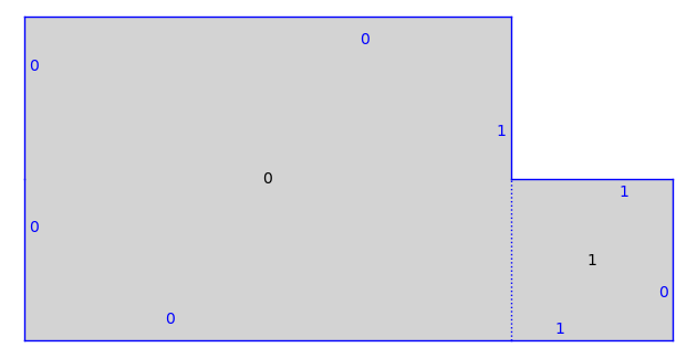
We can also create a half-translation surface:
T = MutableOrientedSimilaritySurface.from_surface(S)

T.glue((1, 1), (0, 2))
T.glue((0, 4), (0, 5))
T.set_immutable()

print(T)
T.plot()
Half-Translation Surface in Q_1(2, -1^2) built from a square and a rectangle
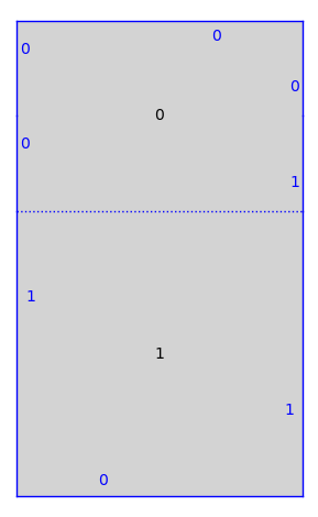
Or anything that can be built by gluing with similarities…
T = MutableOrientedSimilaritySurface.from_surface(S)

T.glue((0, 0), (1, 1))
T.glue((0, 5), (0, 3))
T.set_immutable()

print(T)
T.plot()
Genus 2 Surface built from a square and a rectangle
There is a relatively small contract that a surface needs to implement, things such as “what is on the other side of this edge?”, “is this surface compact?”, … so it is not too hard to implement infinite type surfaces from scratch.
Further Reading
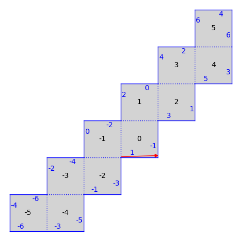
Trajectories & Saddle Connections
Starting from a tangent vector, we can shoot a trajectory along that tangent vector. The trajectory will stop when it hits a singularity of the surface or after some (combinatorial) limit has been reached.
from flatsurf import translation_surfaces

S = translation_surfaces.infinite_staircase()
T = S.tangent_vector(0, (1/47, 1/49), v=(1, 1/31))

S.plot() + T.plot(color="red")
trajectory = T.straight_line_trajectory()
trajectory.flow(100)

S.plot() + trajectory.plot(color="red")
Note that on a finite type surface, we can compute a FlowDecomposition (see below) to determine how a surface decomposes in a direction into areas with periodic and dense trajectories.
We can also determine all the saddle connections up to a certain length bound (on finite type surfaces.)
from flatsurf import translation_surfaces
S = translation_surfaces.octagon_and_squares()

connections = S.saddle_connections(squared_length_bound=50)

# To get a more interesting picture, we color the saddle connections according to their length.
lengths = sorted(set(c.length() for c in connections))
color = lambda connection: colormaps.Accent(lengths.index(connection.length()) / len(lengths))[:3]

S.plot(polygon_labels=False, edge_labels=False) + sum(sc.plot(color=color(sc)) for sc in connections)
Further Reading
Supported Base Rings
Surfaces can be defined over most exact subrings of the reals from SageMath.
Here is an example defined over a number field:
from flatsurf import similarity_surfaces, Polygon

P = Polygon(angles=(1, 1, 4), vertices=[(0, 0), (1, 0)])
S = similarity_surfaces.billiard(P).minimal_cover(cover_type="translation")

print(S.base_ring())
S.plot(polygon_labels=False, edge_labels=False)
Number Field in c with defining polynomial x^2 - 3 with c = 1.732050807568878?
Here is a surface with a transcendental coordinate, supported through exact-real.
from pyexactreal import ExactReals

R = ExactReals(QuadraticField(3))
almost_one = R.random_element(1)

almost_one
/usr/share/miniconda3/envs/test/lib/python3.11/site-packages/cppyy/__init__.py:341: DeprecationWarning: pkg_resources is deprecated as an API. See https://setuptools.pypa.io/en/latest/pkg_resources.html
  import pkg_resources as pr
ℝ(1=2305843009213694107p-61 + ℝ(0.303644…)p-64)
from flatsurf import similarity_surfaces, Polygon

P = Polygon(angles=(1, 1, 4), vertices=[(0, 0), (almost_one, 0)])
S = similarity_surfaces.billiard(P).minimal_cover(cover_type="translation")

print(S.base_ring())
S.plot(polygon_labels=False, edge_labels=False)
Real Numbers as (Real Embedded Number Field in a with defining polynomial x^2 - 3 with a = 1.732050807568878?)-Module
Flow Decompositions
We compute flow decompositions on the unfolding of the (2, 2, 5) triangle. We pick some direction coming from a saddle connection and decompose the surface into cylinders and minimal components in that direction.
from flatsurf import similarity_surfaces, Polygon
P = Polygon(angles=(2, 2, 5))
S = similarity_surfaces.billiard(P).minimal_cover(cover_type="translation")

G = S.graphical_surface(polygon_labels=False, edge_labels=False)
connection = next(iter(S.saddle_connections(squared_length_bound=4)))

G.plot() + connection.plot(color="red")
from flatsurf import GL2ROrbitClosure

O = GL2ROrbitClosure(S)
decomposition = O.decomposition(connection.holonomy())

decomposition
FlowDecomposition with 4 cylinders, 0 minimal components and 0 undetermined components
In this direction, the surface decomposes into 4 cylinders. Currently, sage-flatsurf cannot plot these cylinders. The optional ipyvue-flatsurf widgets can be used to visualize these cylinders in a Jupyter notebook.
from ipyvue_flatsurf import Widget
Widget(decomposition)
Here is a somewhat mysterious case. On the same surface, trying to decompose into a direction of a particular saddle connection, we can never certify that the components is minimal. (We ran this for a very long time and there really don’t seem to be any cylinders out there.)
c = P.base_ring().gen()
direction = (12*c^4 - 60*c^2 + 56, 16*c^5 - 104*c^3 + 132*c)

O = GL2ROrbitClosure(S)
decomposition = O.decomposition(direction, limit=1024)

decomposition
FlowDecomposition with 0 cylinders, 0 minimal components and 1 undetermined components
We can also see the underlying Interval Exchange Transformation, to try to understand what is going on here.
O.decomposition(direction, limit=0).components()[0R].intervalExchangeTransformation()
[9: (28*c^5 - 148*c^3 + 160*c ~ 14.261238)] [14: (-64*c^5 + 356*c^3 - 412*c ~ 11.590863)] [12: (8*c^5 - 48*c^3 + 68*c ~ 4.3066573)] [22: (40*c^5 - 216*c^3 + 236*c ~ 0.074809782)] [21: (12*c^5 - 68*c^3 + 84*c ~ 1.5704962)] [19: (-116*c^5 + 644*c^3 - 744*c ~ 16.873760)] [26: (268*c^5 - 1500*c^3 + 1788*c ~ 4.3783334)] [24: (-248*c^5 + 1388*c^3 - 1652*c ~ 0.54856131)] [18: (40*c^5 - 216*c^3 + 236*c ~ 0.074809782)] [7: (16*c^5 - 88*c^3 + 104*c ~ 6.7127970)] / [7] [22] [24] [26] [19] [21] [18] [12] [14] [9]
Further Reading
the
module referencefor computations related to the \(GL_2(\mathbb{R})\)-orbit closure
\(SL_2(\mathbb{Z})\) orbits of square-tiled Surfaces
Square-tiled surfaces (also called origamis) are translation surfaces built from unit squares. Many properties of their \(GL_2(\mathbb{R})\)-orbit closures can be computed easily.
Note that the Origami object that we manipulate below are different from all other translation surfaces that were built above (that were using sage-flatsurf.)
from surface_dynamics import Origami

O = Origami('(1,2)', '(1,3)')

O.plot()
T = O.teichmueller_curve()
T.sum_of_lyapunov_exponents()
4/3
O.lyapunov_exponents_approx()
[0.333868318977939]
The stratum of this surface and the stratum component.
O.stratum(), O.stratum_component()
(H_2(2), H_2(2)^hyp)
A Database of Arithmetic Teichmüller Curves
There is a relatively big database of pre-computed arithmetic Teichmüller curves that can be queried.
from surface_dynamics import OrigamiDatabase

D = OrigamiDatabase()

D.info()
genus 2
=======
 H_2(2)^hyp        : 205 T. curves (up to 139 squares)
 H_2(1^2)^hyp      : 452 T. curves (up to 80 squares)

genus 3
=======
 H_3(4)^hyp        : 163 T. curves (up to 51 squares)
 H_3(4)^odd        : 118 T. curves (up to 41 squares)
 H_3(3, 1)^c       :  72 T. curves (up to 25 squares)
 H_3(2^2)^hyp      : 280 T. curves (up to 33 squares)
 H_3(2^2)^odd      : 390 T. curves (up to 30 squares)
 H_3(2, 1^2)^c     : 253 T. curves (up to 20 squares)
 H_3(1^4)^c        : 468 T. curves (up to 20 squares)

genus 4
=======
 H_4(6)^hyp        : 118 T. curves (up to 25 squares)
 H_4(6)^odd        :  60 T. curves (up to 18 squares)
 H_4(6)^even       :  35 T. curves (up to 19 squares)
 H_4(5, 1)^c       :  47 T. curves (up to 15 squares)
 H_4(4, 2)^odd     :  61 T. curves (up to 16 squares)
 H_4(4, 2)^even    :  96 T. curves (up to 16 squares)
 H_4(4, 1^2)^c     : 100 T. curves (up to 14 squares)
 H_4(3^2)^hyp      : 197 T. curves (up to 21 squares)
 H_4(3^2)^nonhyp   : 140 T. curves (up to 16 squares)
 H_4(3, 2, 1)^c    :  26 T. curves (up to 14 squares)
 H_4(3, 1^3)^c     :  58 T. curves (up to 14 squares)
 H_4(2^3)^odd      : 151 T. curves (up to 16 squares)
 H_4(2^3)^even     : 170 T. curves (up to 17 squares)
 H_4(2^2, 1^2)^c   : 139 T. curves (up to 13 squares)
 H_4(2, 1^4)^c     :  27 T. curves (up to 13 squares)
 H_4(1^6)^c        :  43 T. curves (up to 12 squares)

genus 5
=======
 H_5(8)^hyp        : 106 T. curves (up to 19 squares)
 H_5(8)^odd        :  26 T. curves (up to 13 squares)
 H_5(8)^even       :  33 T. curves (up to 13 squares)
 H_5(7, 1)^c       :  10 T. curves (up to 12 squares)
 H_5(6, 2)^odd     :  20 T. curves (up to 13 squares)
 H_5(6, 2)^even    :  30 T. curves (up to 13 squares)
 H_5(6, 1^2)^c     :  19 T. curves (up to 12 squares)
 H_5(5, 3)^c       :   9 T. curves (up to 12 squares)
 H_5(5, 2, 1)^c    :  18 T. curves (up to 12 squares)
 H_5(4^2)^hyp      : 127 T. curves (up to 17 squares)
 H_5(4^2)^odd      : 113 T. curves (up to 13 squares)
 H_5(4^2)^even     : 128 T. curves (up to 13 squares)
 H_5(4, 3, 1)^c    :  14 T. curves (up to 12 squares)
 H_5(4, 2^2)^odd   :  29 T. curves (up to 12 squares)
 H_5(4, 2^2)^even  :  27 T. curves (up to 12 squares)
 H_5(3^2, 2)^c     :  27 T. curves (up to 12 squares)

genus 6
=======
 H_6(10)^hyp       :  46 T. curves (up to 15 squares)
 H_6(10)^odd       :   4 T. curves (up to 11 squares)
 H_6(10)^even      :  33 T. curves (up to 12 squares)


Total: 4688 Teichmueller curves
The properties that are stored for each curve.
D.cols()
['representative',
 'stratum',
 'component',
 'primitive',
 'quasi_primitive',
 'orientation_cover',
 'hyperelliptic',
 'regular',
 'quasi_regular',
 'genus',
 'nb_squares',
 'optimal_degree',
 'veech_group_index',
 'veech_group_congruence',
 'veech_group_level',
 'teich_curve_ncusps',
 'teich_curve_nu2',
 'teich_curve_nu3',
 'teich_curve_genus',
 'sum_of_L_exp',
 'L_exp_approx',
 'min_nb_of_cyls',
 'max_nb_of_cyls',
 'min_hom_dim',
 'max_hom_dim',
 'minus_identity_invariant',
 'monodromy_name',
 'monodromy_signature',
 'monodromy_index',
 'monodromy_order',
 'monodromy_solvable',
 'monodromy_nilpotent',
 'monodromy_gap_primitive_id',
 'relative_monodromy_name',
 'relative_monodromy_signature',
 'relative_monodromy_index',
 'relative_monodromy_order',
 'relative_monodromy_solvable',
 'relative_monodromy_nilpotent',
 'relative_monodromy_gap_primitive_id',
 'orientation_stratum',
 'orientation_genus',
 'pole_partition',
 'automorphism_group_order',
 'automorphism_group_name']
Some sample queries
The Teichmüller curves in genus \(g\) such that in any direction we have at least \(g\) cylinders.
for g in range(2, 7):
    q = D.query(('genus', '=', g), ('min_nb_of_cyls', '>=', g))
    print(f"g={g}: {q.number_of()}")
g=2: 91
g=3: 37
g=4: 1
g=5: 0
g=6: 0
Some more information than just the count:
g = 3

q = D.query(('genus', '=', g), ('min_nb_of_cyls', '>=', g))

q.cols('stratum')

print(set(q))
{H_3(1^4), H_3(2^2), H_3(2, 1^2)}
The actual Origami representations from the “representative” column.
q.cols('representative')

o = choice(q.list())

print(o)
(1)(2,3,4,5)(6,7,8,9)
(1,2,3,6)(4,7,9,8)(5)
Further Reading
Combinatorial Graphs up to Isomorphism
We list the graphs of genus 2 with 2 faces and vertex degree at least 3.
from surface_dynamics import FatGraphs

graphs = FatGraphs(g=2, nf=2, vertex_min_degree=3)

len(graphs.list())
21819
One such graph in the list:
graphs.list()[0]
FatGraph('(0,9,8,6,5,7,4,2,1,3)', '(0,2,1,3,4,6,5,7,8)(9)')
Further Reading
Hyperbolic Geometry
sage-flatsurf provides an implementation of hyperbolic geometry that unlike the one in SageMath does not rely on the symbolic ring.
We define the hyperbolic plane over a number field containing a third root of 2.
from flatsurf import HyperbolicPlane

K.<a> = NumberField(x^3 - 2, embedding=1)

H = HyperbolicPlane(K)
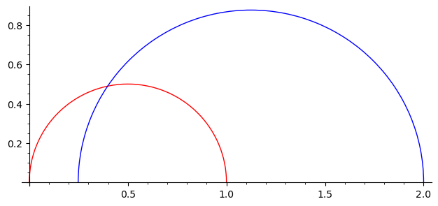
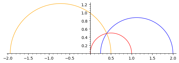
We plot some geodesics in the upper half plane and in the Klein model.
g = H.geodesic(0, 1)
h = H.geodesic(1/2 - a/5, 2)

g.plot(color="red") + h.plot(color="blue")
g.plot(model="klein", color="red") + h.plot(model="klein", color="blue")
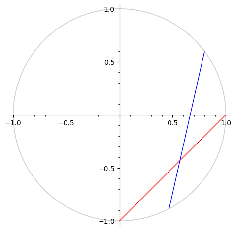
We determine the point of intersection of these geodesics. Note that that point has no coordinates in the upper half plane (without going to a quadratic extension.)
P = g.intersection(h)
P.coordinates(model="klein")
(-480/15193*a^2 - 2000/15193*a + 11924/15193,
 -480/15193*a^2 - 2000/15193*a - 3269/15193)
P.change_ring(AA).coordinates(model="half_plane")
(0.3974561732377553?, 0.4893718050653866?)
We use that point to define another geodesic to the infinite point ½.
g.plot(color="red") + h.plot(color="blue") + H.geodesic(P, 1/2).plot(color="orange")
Further Reading
the
module referencefor hyperbolic geometry
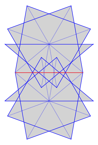
Veech Surfaces
We can explore how a Veech surfaces decomposes into cylinders.
from flatsurf import polygons, similarity_surfaces, GL2ROrbitClosure

T = polygons.triangle(1, 4, 7)
S = similarity_surfaces.billiard(T).minimal_cover('translation')
S = S.erase_marked_points()

S.plot()
O = GL2ROrbitClosure(S)
decomposition = O.decomposition((1, 0))

decomposition
FlowDecomposition with 4 cylinders, 0 minimal components and 0 undetermined components
bool(decomposition.parabolic()) # the underlying value is a tribool, since it could be undetermined
True
Further Reading
the
module referencerelated to the \(GL_2(\mathbb{R})\)-orbit closure
Strata & Orbit Closures
We can query the stratum a surface belongs to, and then (often) determine whether the surface has dense orbit closure.
from flatsurf import similarity_surfaces, polygons

T = polygons.triangle(2, 3, 8)
S = similarity_surfaces.billiard(T).minimal_cover('translation')

S.stratum()
H_6(7, 2, 1)
from flatsurf import GL2ROrbitClosure

O = GL2ROrbitClosure(S)
O
GL(2,R)-orbit closure of dimension at least 2 in H_6(7, 2, 1) (ambient dimension 14)
for decomposition in O.decompositions(10, limit=20):
    if O.dimension() == O.ambient_stratum().dimension():
        break
    O.update_tangent_space_from_flow_decomposition(decomposition)

O
GL(2,R)-orbit closure of dimension at least 14 in H_6(7, 2, 1) (ambient dimension 14)
Further Reading
the
module referencerelated to the \(GL_2(\mathbb{R})\)-orbit closure
Veering Triangulations
We create a Veering triangulation from the stratum \(H_2(2)\).
from veerer import VeeringTriangulation, FlatVeeringTriangulation
from surface_dynamics import Stratum

H2 = Stratum([2], 1)
VT = VeeringTriangulation.from_stratum(H2)

VT
VeeringTriangulation("(0,6,~5)(1,8,~7)(2,7,~6)(3,~1,~8)(4,~2,~3)(5,~0,~4)", "RRRBBBBBB")
If you aim to study a specific surface, you might need to input the veering triangulation manually.
triangles = "(0,~7,6)(1,~5,~2)(2,4,~3)(3,8,~4)(5,7,~6)(~8,~1,~0)"
edge_slopes = "RBBRBRBRB"
VT2 = VeeringTriangulation(triangles, edge_slopes)

VT2
VeeringTriangulation("(0,~7,6)(1,~5,~2)(2,4,~3)(3,8,~4)(5,7,~6)(~8,~1,~0)", "RBBRBRBRB")
VT2.stratum()
/usr/share/miniconda3/envs/test/lib/python3.11/site-packages/surface_dynamics/flat_surfaces/abelian_strata.py:238: UserWarning: AbelianStratum has changed its arguments in order to handle meromorphic and higher-order differentials; use Stratum instead
  warnings.warn('AbelianStratum has changed its arguments in order to handle meromorphic and higher-order differentials; use Stratum instead')
H_2(2)
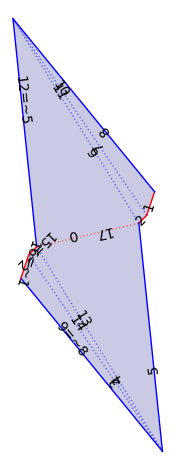
We play with flat structures on a Veering triangulation. There are several pre-built constructions.
F0 = VT.flat_structure_middle()
F0.plot()
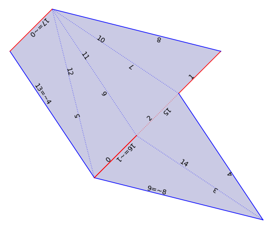
F1 = VT.flat_structure_geometric_middle()
F1.plot()
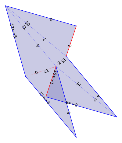
F2 = VT.flat_structure_min()
F2.plot()
We can work with \(L^{\infty}\)-Delaunay flat structures. These are also called geometry flat structures in veerer.
We check that the Veering triangulation VT corresponds to an open cell of the \(L^\infty\)-Delaunay decomposition of \(H_2(2)\).
VT.is_geometric()
True
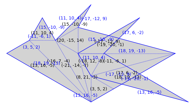
We compute the cone of \(L^\infty\)-Delaunay data for the given Veering triangulation VT.
Each point in the cone corresponds to a geometric flat structure given as \((x_0, \ldots, x_8, y_0, \ldots, y_8)\) where \((x_i, y_i)\) is the holonomy of the \(i\)-th edge.
The geometric structure is a polytope. Here the ambient dimension 18 corresponds to the fact that we have 9 edges (each edge has an \(x\) and a \(y\) coordinate.) The dimension 8 is the real dimension of the stratum (\(\dim_\mathbb{C} H_2(2) = 4\).)
geometric_structures = VT.geometric_polytope()

geometric_structures
Cone of dimension 8 in ambient dimension 18 made of 10 facets (backend=ppl)
The rays allow to build any vector in the cone via linear combination (with non-negative coefficients).
rays = list(map(QQ**18, geometric_structures.rays()))
If all entries are positive, we have a valid geometric structure on VT.
xy = rays[0] + rays[12] + rays[5] + 10 * rays[6] + rays[10] + rays[16]

xy
(13, 1, 1, 17, 16, 3, 16, 17, 18, 3, 3, 1, 25, 26, 29, 26, 25, 22)
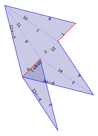
Construct the associated flat structure (note that x and y are inverted.)
flat_veering = VT._flat_structure_from_train_track_lengths(xy[9:], xy[:9])

flat_veering.plot()
We now explore the \(L^\infty\)-Delaunay of a given linear family.
We do it for the ambient stratum, i.e., the tangent space is everything.
The object one needs to start from is a pair of a Veering triangulation and a linear subspace.
L = VT.as_linear_family()
The geometric automaton is the set of such pairs that one obtains by moving around in the moduli space.
Initially, there is only the pair we provided.
A = L.geometric_automaton(run=False)

A
Partial geometric veering linear constraint automaton with 1 vertex
A.run(10)

A
Partial geometric veering linear constraint automaton with 11 vertices
We could compute everything (until there is nothing more to be explored).
If the computation terminates, it proves that L was indeed the tangent space to a \(GL_2(\mathbb{R})\)-orbit closure.